Multispectral Image Analysis in a Docker Container: Examples (continued)
Starting the Container
To recap:
sudo docker run -d -p 433:8888 -v yourImageFolder:/crc/imagery --name=crc mort/crcdocker
then point your browser to
http:\localhost:433
Note: If you are running Docker on Linux in VMWare Player on a Windows host in NAT mode, run the browser in the VM as well. If you are in Bridged mode and in a LAN, you can connect to the IPython kernel from your Windows browser by finding the address of the VM (for example in your Router status) and replacing localhost with that address.
Example 3: Solar Illumination Correction in Rough Terrain
Topographic modeling can be used to correct images for the effects of local solar illumination. The local illumination depends not only upon the sun's position (elevation and azimuth) but also upon the slope and aspect of the terrain being illuminated. The Figure below shows the angles involved.
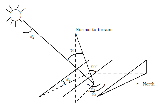 Figure 1 Angles involved in computation of local solar incidence: \(\theta_z=\) solar zenith angle, \(\phi_a=\) solar azimuth, \(\theta_p=\) slope, \(\phi_o=\) aspect, \(\gamma_i=\) local solar incidence angle.
The quantity to be determined is the local solar incidence angle \(\gamma_i\), which determines the local irradiance. From trigonometry we can calculate the relation \[ \cos\gamma_i = \cos\theta_p\cos\theta_z + \sin\theta_p\sin\theta_z\cos(\phi_a-\phi_o). \] For a Lambertian surface, the reflected radiance \(L_H\) from a horizontal surface toward a sensor (ignoring all atmospheric effects) is given by \[ L_H = E\cdot\cos\theta_z\cdot R. \] For a surface in rough terrain the reflected radiance \(L_T\) is similarly \[ L_T = E\cdot\cos\gamma_i\cdot R, \] thus giving the standard cosine correction relating the observed radiance \(L_T\) to that which would have been observed had the terrain been flat, namely \[ L_H = L_T{\cos\theta_z\over\cos\gamma_i}. \] The Lambertian assumption is in general a poor approximation, the actual reflectance being governed by a bidirectional reflectance distribution function (BRDF), which describes the dependence of reflectance on both illumination and viewing angles as well as on wavelength. Particularly for the large range of incident angles involved with rough terrain, the cosine correction will over- or underestimate the extremes and lead to unwanted artifacts in the corrected imagery.
An example of an approach which takes better account of BRDF effects is the semiempirical cosine correction (C-correction) method. We replace Equations above for \(L_H\) and \(L_T\) by \[
L_H = m\cdot \cos\theta_z + b, \quad L_T = m\cdot \cos\gamma_i + b.
\] The empirical parameters \(m\) and \(b\) can be estimated from a linear regression of observed radiance \(L_T\) vs.
\(\cos\gamma_i\) for a particular image band. Then, we can write \[
L_H = L_T\left({\cos\theta_z + b/m\over \cos\gamma_i + b/m}\right)
\] as a correction formula.
The main difficulty with this method is estimating the slope \(m\) and intercept \(b\) reliably since the natural spread in ground reflectance will tend to mask any correlation with local solar incidence angle. The approach adopted here is to precede the calculation with an unsupervised segmentation of the image into a small number of land-cover classes and then to estimate the regression coefficients separately for each class and each spectral band. Only if the correlation exceeds a threshold (0.2) are the image pixels corrected. Here is the bash script which controls the correction process:
cat /crc/c-correction.sh
A selected spatial/spectral subset of the image to be corrected is first of all subjected to a principal components analysis (with the Python script pca.py). Then the first three principal components are passed to the Gaussian mixture clustering script em.py. The resulting class image is then fed to the c-correction program proper (c_corr.py) along with the original image and the DEM. The class labels then act as masks, with the c-correction being applied to each class separately. We'll try it out here with a Landsat 5 TM image acquired over the southeastern part of Vancouver Island, Canada, in July, 1984. The footprint of the spatial subset chosen is shown below.
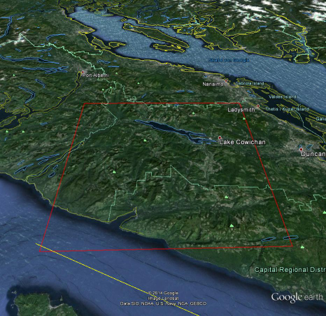 Figure 2 Footprint of the Landsat 5 TM spatial subset projected onto Google Earth.
Here is an RGB composite of bands 4,5 and 7:
run dispms -f imagery/19840717 -p [4,5,7] -d [3154,3122,2000,2000]

We choose three land-use classes and the non-thermal bands 1,2,3,4,5 and 7 and run the bash script:
!./c-correction.sh [3154,3122,2000,2000] [1,2,3,4,5,7] 3 132.9 54.9 imagery/19840717 imagery/dem_utm
Examining the above output we see that pixel intensities in class 2 always have a very low correlation with the local incidence angle so that no correction is applied. For bands 1 through 4, classes 1 and 3 are corrected, whereas for bands 5 and 7 only class 1 pixels exhibit a strong enough correlation to warrant the c-correction. In fact class 2 corresponds to low-lying areas and water surfaces as can be seen here in a linear stretch of the class image (class 1 = black, class 2 = gray, class 3 = white, the \(\cos(\gamma_i)\) image is shown for camparison on the right).
run dispms -f imagery/19840717_pca_em -F imagery/COSGAMMA -e 2 -E 4

The effect of the illumination correction can be seen clearly in band 4, first for the full subset:
run dispms -f imagery/19840717_corr -p [4,4,4] -e 3 -F imagery/19840717 -D [3154,3122,2000,2000] -P [4,4,4]


And for a \(1000\times 1000\) subset at the lower left:
run dispms -f imagery/19840717_corr -p [4,4,4] -d [0,800,1000,1000] -e 3 -F imagery/19840717 -D [3154,3922,1000,1000] -P [4,4,4]
